He's Outta Here...

I leave for Costa Rica tomorrow afternoon. I'll be back around the 20th of January, after three solid weeks of tropical fun, birding and herping with no one to answer to. It's going to be great. That means you won't see any further posts here until late January. Until then, have a good one!

Happy Holidays!

Nick

Top 10 Nature Moments of 2007

If 10,000 Birds and The Hawk Owl's Nest can do it, so can I. Here are my personal Top 10 Nature Moments of 2007.

10. All four Longspurs in a year!

Starting with a vagrant Smith's Longspur with Laplands on Long Island early this year, I managed to be successful in seeing all four Longspurs when I found both McKay's and Chestnut-colored in Wyoming in August.

9. A long-time nemesis falls: Nelson's Sharp-tailed Sparrow

I blog this really cool species again and again and again, looking at both subspecies identification and the reasons for the Nelson's / Saltmarsh species split.

8. Stadium Birding

Stadium birding is always a hit. Especially when you get to watch 19 Warbler species and 42 species total... at 1am.

7. Montezuma Muckrace

I competed in the Montezuma Muckrace for the third time this fall, for the second time with one of two student teams from Cornell. This year, my team managed to place third, tied with Chris Tessaglia-Hymes's team with 122 species. The after-action report from the Muckrace indicated that our team raised $265 and the Muckrace total raised a record high amount of over $10k!

6. I fall in love with Red-bellies!

I got a herp lifer, Red-bellied Snake (Storeria occipitomaculata), promptly found about 30 more over the course of the summer, and have absolutely fallen in love.

5. Allegany State Park herping

My band of herping friends and I traveled to Allegany State Park, pulling down a whopping total of 25 species in a weekend, with four lifers including the stunning Long-tailed Salamander (Eurycea longicauda).

4. My NY big year in herps - 40 species total

I never got to writing a summary post on my unofficial herping big year in NY, but it was big!

14 species of salamander (4 lifers)
11 species of frog (2 lifers)
3 species of turtle (a lifer subspecies)
1 species of lizard (a lifer)
11 species of snake (6 lifers)

For a total of 40 species and 13 lifers! Not bad at all for NY, even though I had some major misses.

Selected herping posts:
Spring Field Survey (Black Rat Snake)
Allegany State Park (Long-tailed Salamander, Wehrle's Salamander, Short-headed Garter)
Green Snake and Coal Skink
Massasauga
Sniffing Mink Frogs in the Adirondacks
Long Island Herping (Marbled Salamander, Ribbon Snake)


3. Winter Finches!

Certainly the highlight of NY birding this year has been the Winter Finch Invasion! We in the Cayuga Lake Basin have finally completed the Winter Finch Sweep (although I have not, personally - I still need Hoary Redpoll and White-winged Crossbill... as lifers!).

Select posts:

Seeing those finches for myself
Where are the Bohemian Waxwings?
Pinicola!
Enucleator!
Patterns of Winter Irruptives

2. TAing my Field Biology Class... in the Field!

This semester I was a Teaching Assistant for Introductory Field Biology with my mentor, Charlie Smith. It was a ton of fun! See my posts on herps, fish, mammals, and more here.

1. Colorado-Wyoming-AOU Trip! 55 bird lifers and 11 herp lifers in 8 days!

The series of 10 posts begins here. Photo-heavy and lots of fun!

In the Lab 5: Data Analysis and Results

Last in my series of posts on phylogenetic research. See Parts 1, 2, 3, and 4.

This is where I admit I'm getting cheap on you, for several reasons. The first - I haven't completely finished my own results, and I won't be posting them here because they are intended for publishing. The second - I am still a student and not a master of phylogenetic analysis, so to speak. I am only acquainted with a couple of analysis methods, which I will describe here. Third - I am really running out of time, as I depart for winter break in Costa Rica in just four days. I will, when I return next semester, be able to give a more complete summary of the different analyses of phylogeography. For now, you get Analysis Lite.

We started off with an idea for a study and birds in the field. We've collected blood from those birds, purified DNA, PCR'ed, sequenced, and cleaned up the data. Now we have our completed data set: sequences for multiple loci, from individual Palm-Tanagers across Hispaniola. Remember from Part 1 that our sampling consisted of up to five individuals from sites across Hispaniola:

The most basic level of analysis I use is called statistical parsimony haplotype networks. These networks, constructed using a program called TCS. These networks are a phlyogenetic reconstruction of relationships for any given locus. Unlike trees, the networks allow a more reticulated relationship. Trees force each individual to a terminal branch, networks are used when relatedness is higher and there can be ancestral alleles still present. It is a nifty way of visualizing a complicated network of genetic similarity. A simple example follows:

In the above example, the network consists of ~30 individuals. The color-filled circles each represent a unique haplotype (a unique DNA sequence). Each haplotype's circle is sized proportional to how many individuals share that haplotype. The smallest colored circles have only one individual with that haplotype, the large central circle has ~15 individuals sharing an identical sequence. The lines and black nodes that connect the network together represent the relationships of the DNA sequence. Each line separating haplotypes represent one base pair change. The black nodes represent inferred ancestral alleles, intermediate haplotypes that are no longer present. For example: the smallest red circle on the left differs from the larger red circle by four base pairs. The two red circles directly next to each other differ by one base pair. Finally, to complete the analysis, the colors are representative of the locality each individual comes from (they correspond in this example to the map above). Thus the most well-represent haplotype above is shared by ~15 individuals from 6 localities above.

Analysis of haplotype networks is quite simple: you just eyeball it. In the example above, there seem to be two distinct groups separated by six base pair changes. One group is solely of individuals from the red locality, on the western Peninsula on the map above. The other consists of a mix of every other locality on the island sampled. Note in particular that in this second group, every locality is represented in the single central haplotype. This is indicative of panmixia - there are no barriers to gene flow between these localities. We can infer that there is some barrier of gene flow separating the red population from the rest (although in the example network sample sizes are very low, this may skew the analysis by missing rarer alleles that may connect the populations). These two clades (red/everything else) are reciprocally monophyletic, the buzzword of genetic studies. Individuals from the red location do not occur in the other clade, and vice versa. Reciprocal monophyly, especially with large sample sizes, is a very strong indication of a lack of gene flow between populations.

Now that you have a handle on haplotype networks, check out this example of a more complicated network:

(Source)

Looking at how phylogenetic breaks - such as the monophyletic red clade identified above, overlay with topography is the basis of phylogeography. It allows us to identify likely topographic barriers to gene flow that allowed population isolation and differentiation, although it is important to note that we can infer barriers but this study is itself not a test of that barrier.

There are more detailed methods of analysis, such as tree-based phylogenetic reconstruction. I also intend to use an analysis called Isolation with Migration that generates a likely model of of the isolation of distinct clades, with migration rates between them.

When all is done, I hope to turn my poster from the AOU meeting into a published paper:

Now, just so you don't feel completely let down (all method and no results!) I will cover some of our group's work that was recently published this year. All of the methods of study I am applying to the Palm-Tanagers, Andrea has already done for the Chat-Tanagers (Calyptophilus). These two species, unlike the Palm-Tanagers, are high-elevation specialists, being found in the mountain ranges on Hispaniola.

Eastern Chat-Tanager (Calyptophilus frugivorous)

Photo courtesy of Andrea Townsend

Chat-Tanager ranges and sample locations (click for detail)

The haplotype networks for four loci (mtDNA ND2 and three nuclear introns) follow. Locality colors correspond to the above map. 48 samples total. Click to enlarge.

(Figures from Townsend et al. 2007)

A brief glance at the four networks will indicate the general trend: two distinct clades corresponding to the red/orange/yellow western localities and the blue/green/purple eastern localities. The genus has been considered by various sources as anywhere from one to four species, this work pretty much solidifies the taxonomy as two distinct species. The mitochondrial DNA ND2 gene is most telling - the black bar separating the two clades indicates approximately 100 base pair substitutions, giving the two species approximately 12% uncorrected divergence for this mtDNA locus. This is a very large, ancient difference - with the standard avian molecular clock and the IM analysis indicates the taxa diverged approximately 9 million years ago.

The nuclear introns show the same pattern as the mtDNA, but with much less actual divergence (1-2%). Also, two of the introns are not reciprocally monophyletic, with a handful or rare alleles falling in the 'wrong' clade. This may indicate a very limited amount of gene flow between the two species.

Within each respective clade, there is no population structure at all. As in the simple example I explained above, all localities are represented in the common haplotypes with few outliers. This indicates that gene flow among the populations within each species is common.

We can now examine what topographic barriers may be important. Recall the topography of Hispaniola and compare it with the species range maps above.

(Source)

The mountain-dwelling Calyptophilus occur in distinct populations in each of the distinct east-west mountain ranges. We have two distinct clades encompassing several mountain ranges each. There may be limited gene flow between the two clades, but there is no structure within either population. This indicates that, despite the high-elevation specialist populations being separated by deep valleys and long distances, disjunct mountain ranges do not present a barrier to gene flow in either species. If the mountains aren't a cause for the divergence and speciation of Calyptophilus on Hispaniola, what is?

Recall two things: the ancient divergence of 9 million years, and the paleohistoric tendency of the intermontane valleys to flood. In fact, Hispaniola 15 million years ago consisted of two paleo-island blocks, which merged approximately 9 million years ago to form the island we know today. The divide between two island blocks is the deep (below sea level) valley that separates the southwestern peninsula from the rest of the island (the green area with the large lagoons in the topo map, the heavier red line in the species range map). This region is the area the two species come into contact. These facts suggest that Calyptophilus diverged not on the single island of Hispaniola, but they diverged allopatrically on two separate paleo-island blocks. Back in Part 1 we began this study to see if Hispaniola was big enough to support in situ speciation. The evidence from Calyptophilus phylogeography suggests that it is not.

Look for me to be writing more when I have results from the rest of the endemic species pairs on Hispaniola! This concludes my series, I hope you enjoyed it.

Reference:

Andrea K. Townsend, Christopher C. Rimmer, Steven C. Latta, and Irby J. Lovette. 2007. Ancient differentiation in the single-island radiation of endemic Hispaniolan chat-tanagers (Aves: Calyptophilus). Molecular Ecology. 16: 3634-3642. (Abstract)

In the Lab 4: From DNA to Data (2)

Fourth post on lab methods in my phylogeography study - see Parts 1, 2, and 3.

We have now collected blood from the bird in the field, purified a DNA sample from that blood, and amplified billions of copies of a target locus from that DNA. The next step, the second step heavy in biochemistry, is reading the sequence of that DNA strand.

The sequencing method now widely used is known as dye-terminator sequencing, and is a derivation of the original Sanger sequencing. The process begins with a reaction that is mechanistically much the same as PCR, with a series of three-step temperature cycles to create and elongate new DNA strands. This time, ddNTPs (dideoxynucleotide triphosphate) are added to the mixture of dNTPs (deoxynucleotide triphosphate). These nucleotides are identical to those normally used in DNA elongation, except that they lack the -OH hydroxyl group used by the polymerase to add the next nucleotide in the sequence. Thus, when added they terminate the sequence. These ddNTPs have a fluorescent dye attached, with a different color of fluorescence for each base (A, T, C, G), which will be used later to actually read the sequence. The ddNTPs are added in much smaller concentrations than the dNTPs, so the cycling produces a variety of lengths of sequence, depending on when a ddNTP happens to be added instead of a dNTP. Finally, another difference from PCR is the primer mixture used. In the sequencing reaction, only one primer is added to the mixture, instead of both the forward and reverse primers being added. The reason for this will become clear later.

An animated image of the sequencing reaction can be found here.

What results from this process is a mixture of fragments that start with either the forward or reverse primer, proceed in the direction of the primer for a random length, and terminate in a dye-labeled ddNTP. The number of new fragments produced in the sequencing reaction is not nearly as much as in regular PCR, even when run for 30 cycles. This is because only one primer is used at a time during the reaction. The reaction can only proceed in one direction, and the number of copies produced increases linearly rather than exponentially. Thus, the exponential amplification of the locus in PCR beforehand is needed to generate enough copies for the sequencer to read.

The sequencer

Above is our lab's sequencer, a small unit that can only run sixteen samples at a time. We generally run our sequencing at another lab on campus, which has sequencers that can run whole 96-well plates at a time, taking about 3 hours. The samples from the sequencing reaction are mixed into a kind of gel and are read by the sequencer in a process similar to gel electrophoresis. Remember the sample produced in the sequencing reaction is a mixture of fragments of varying lengths. Given the number of copies involved, fragments exist for every length out to several hundred base pairs. When an electrical current is applied, the negative charge of DNA acts to pull it towards the positive node.

The sequencer pulls the DNA fragments through a gel in a tiny capillary tube. The smaller fragments travel faster and farther through the gel. This organizes the fragment mixture pulled through the capillary by length, smallest first. At the end of the capillaries, there is a small sensor that reads the wavelength of fluorescence of the gel. By the time the fragments go past the sensor, they have been pulled into discrete clusters and the sensor reads a peak of color. Thus the first fragment (label on base pair 1) is read, then the second fragment (label on base pair 2), and so on until out of fragments.

Capillaries for 16 samples

The sequencer's all-important sensor

What this process boils down to: reading DNA sequence is as simple as labeling each base pair with a particular color, and drawing the strand past a sensor that reads the color. The sequencer outputs the data to a computer. Using programs such as Sequencher, we then 'clean up the data' for analysis. The output looks as follows:

(Crop from Source)

We can view both the raw data, the colored peaks, and the program's preliminary base 'calls' (its best guess for each peak). 'Cleaning' the data consists of scrolling through the sequence, looking for ambiguous areas caused by dye blobs or other malfunctions. In the example above, the top row of peaks is extremely messy and difficult to call. The bottom row is much cleaner, with well-defined peaks, although there is a very low level of 'noise', the low amounts of blob along the bottom. Too much noise can make the sequence unreadable. Also, true double peaks can occur in heterozygotes, where the two copies of the locus (remember each gene has two copies) differ at a base pair or even a long deletion or insertion. Rerunning the sample will fix most errors; true double peaks can be resolved by cloning (where one copy of the locus is cloned into a bacterium and then sequenced) or by running a program such as PHASE to estimate the sequence of the differing alleles.

Remember I mentioned earlier that a single primer is run in the sequencing reaction, and that both a forward and reverse primer is run for each sample (thus, two sequencing reactions per sample). Besides being necessary for the sequencing reaction to work, this solves two problems in the clean-up phase. The first is length: sequencing reactions generally don't produce fragments the length of the whole locus, so by having two sequences starting the beginning and the end we can reconstruct the whole locus. The second is noise: as the sequencing fragments get longer, the number of copies produced is fewer and thus the quality of the peak read by the sequencer degrades. Having overlapping forward and reverse fragments allows us to call peaks with greater certainty, by having two strands of peaks to call from.

When all of the data is cleaned up, with the ambiguous peaks resolved and any heterozygous alleles identified and sequenced, we now have our data set! We are ready for analysis.

Part 5: Data Analysis and Results

In the Lab 3: From DNA to Data (1)

Third in a post on lab methods in my phylogeography study - see Parts 1 & 2

Raw, purified DNA can be used to analyze sequence data, microsatellites, and more. My phylogeography project uses sequence data from a mitochondrial gene and several nuclear introns. These stretches of DNA sequence range from 500 to 1000 base pairs in length. In order to sequence them, the raw DNA must be chopped into the desired fragments (loci) and amplified by many orders of magnitude. The process that accomplishes this is called PCR: Polymerase Chain Reaction. Prepare your brains for the biochemical heavy lifting of genetic work.

The raw DNA is added to a mixture of the following:

dNTP (deoxyribonucleotide triphosphate) - the nucleotides used to compose the new strands
primers - short sequences of DNA that bind to either end of the locus to be copied
polymerase - the enzyme that binds to the primers and creates the new strands of DNA

The PCR process itself is a series of cycles, each cycle composed of three steps at a different temperature. The first step heats the mixture to roughly 95 degrees C, denaturing and separating the parent DNA strands. The second step cools the mixture to roughly 54 degrees C, and allows the primers and polymerase to bind. A special polymerase, Taq, is needed to withstand the high heat of denaturation without denaturing itself. Taq comes from the heat-tolerant bacteria Thermophilus aquaticus, discovered in Yellowstone hot springs in the 1960's. The third step is intermediate in temperature (72 degrees C), allowing the polymerase to create the new strands by adding nucleotides off the end of the primer.

(Source)

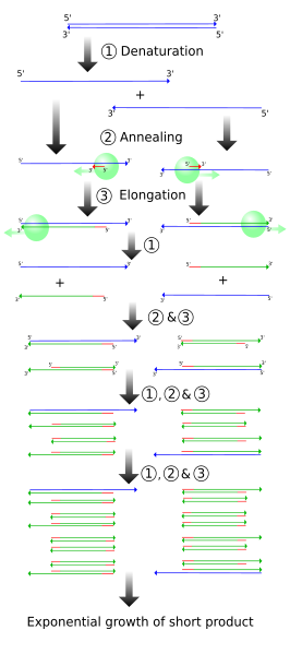
The simplified figure above demonstrates PCR starting with a set-length strand. However, we do PCR on raw DNA. When raw DNA is subjected to PCR, the entire genome is added and only ~1000 base pairs (bp) need to be copied.

How does PCR achieve this? The following figures demonstrates (cropped from the wikipedia source).

One single cycle of the above steps generates two open-ended DNA strands. Each contain the parent strand, along with a new strand that starts with the primer and runs until the step ends. This new strand can be thousands of bp long, depending on how long the extension step is run. Note that the two newly formed strands of DNA are complementary.



Another cycle is completed, generating more open-ended copies from the parent strand. On the open-ended primer strands from cycle 1, the opposite primer binds and adds nucleotides until it reaches the first primer, resulting in a correct-length strand bound to an open-ended strand.



The third cycle creates more open-ended/parent and open-ended/correct-length strands, along with the first replication of the correct-length double strands. Each further cycle allows the number of gene copies to grow exponentially.

Putting it all together, we get the following. Sorry about the poor quality of the cropping, but it was the best representation I could find.

(Source)

These temperature cycles are generated by a Thermocycler. Up to 96 samples are loaded, the exact temperature/time cycle set, and the Thermocycler automates the whole process with tight temperature control. I generally run my samples for about 30 cycles, generating about 2^30 copies of the loci I am sequencing in about 3 hours.

When done, I just run a check with gel electrophoresis to test whether the PCR was successful. I label a small sample of the DNA with dye, run it out on an agarose gel using electrical current (DNA has a negative charge), and view it with UV to highlight the dye. If the PCR was successful, a single bright band will show up of the appropriate length.

UV imaging

If all goes well, I end up with this, rows and rows of PCR product:

With PCR product in hand, literally billions of copies of a locus, we can now sequence it.

Part 4: From DNA to Data (2)

In the Lab 2: From Bird to DNA

To begin a phylogeography study, you need a large amount of genetic data. In my case, I am looking at differences between populations of Palm-Tanagers (Phaenicophilus) - see Part 1.

We get this data by collecting birds from a series of locales across the range of the two species. My study uses around five birds per locale, some studies use far more. Sites were varied, with some in lowlands, and some in the mountains. The intent was to get wide geographic spread and multiple types of topography represented in the samples, as well as to get samples across potential topographic barriers - the large mountain ranges on the island as well as the historic sea channels that once existed.


Bird DNA can be collected by two means. One method is lethal: the collection of a specimen, removal of blood and tissue for analysis, and deposition of a study skin in a museum. Many studies use this method. Although it may seem draconian to kill birds for study, museum specimens provide invaluable reference material for future research. The second method of collection is used in this project: the capture of a bird via mistnet and removal of a blood or feather sample. Avian red blood cells are enucleated, so a large amount of DNA can be recovered from a small blood sample or the tissue remaining in the base of a plucked feather. Museum skins as well can be a source of DNA, from small pieces of skin or toepad clippings. The nonlethal method is used in our work because some of our study birds are endangered, and the birds captured are also part of mark-recapture biodiversity studies.

Taking blood from a Chat-Tanager (Calyptophilus)

(Photo courtesy of Andrea Townsend)

Blood is collected by lightly piercing the vein along the wing with a small needle. A capillary tube is used to suck up the drop of blood created.The blood is transferred to a test tube and treated with blood lysis buffer. This buffer ruptures the blood cells, denatures proteins, and inactivates any enzymes that may denature and destroy the DNA. Thus, the DNA is safeguarded against decay and the blood may be stored in buffer at room temperature for long periods of time.

A blood sample

When all the blood samples required for a study are collected, the rest of the project is completed in the lab. For my study, all the field work was conducted before I joined the project. Thus, I was greeted by this wealth of data:

A whole lotta blood

The next step is to purify DNA from the blood sample. A small sample of the blood is treated with a variety of buffers and reagents, the end result being all of the non-DNA (proteins, membrane fragments, etc) are filtered out and purified DNA remains, as a clear viscous fluid.

Raw genetic material

DNA is purified from all of the blood samples and stored in a -20 degrees F freezer. This pure DNA is the raw material for study from which we can branch off in many directions of research.

On to Part 3: From DNA to Data

In the Lab 1: Island Speciation

My Honor's Thesis is a phylogeography study - the genetic form of biogeography, examining the relationship of phylogenetic lineages and gene flow with geographic distribution. Phylogeography can give us useful insights into speciation and factors influencing biodiversity. My particular study is part of a larger project by Andrea Townsend looking at island speciation on Hispaniola (Haiti and the Dominican Republic). Hispaniola is the second-largest island in the Caribbean, with the highest mountains. Several mountain ranges cleave the island east-to-west, separated by deep alluvial valleys that flood during geological periods of high sea level.

(Source)

Hispaniola is very interesting to birders, as it contains over 30 endemic species and many endemic subspecies. Particularly interesting from an evolutionary perspective is the presence of several sister-species pairs: a pair of species that appear to have diverged from a common ancestor on Hispaniola. Most island speciation is allopatric in nature: species form when a population becomes isolated on the island, diverging and becoming one new species on the island. The presence of multiple sister-species pairs on Hispaniola may indicate that it is large enough to allow avian speciation to occur in situ, something previously only thought to occur on the largest islands (Madagascar, etc).

My study looks at one sister-species pair on the island to examine the effects of past and present topographic barriers on gene flow in the populations. My study species are the Black-crowned Palm-Tanager (Phaenicophilus palmarum) and the Gray-crowned Palm-Tanager (Phaenicophilus poliocephalus), two common habitat-generalist endemics.

Phaenicophilus poliocephalus

(Photo courtesy of Andrea Townsend)

For this study, a large amount of genetic data is needed. The following long-overdue series of posts is a brief step-through of the collection and analysis of genetic data for this type of evolutionary study.

Part 2: From Bird to DNA

Moving Day

I just spent all morning packing up my collection of 22 geckos (2 are my roommate Shawn's) to send them over to LeAnn's house for winter break. As I'll be spending break in the more tropical climate of Costa Rica (7 more days!!!), so LeAnn agreed to watch over things for me. Here's a few photos.

"But I don't wanna move!!!"

22 Geckos, count 'em:
2.2.11 Rhacodactylus ciliatus
0.1 Rhacodactylus auriculatus
0.4 Ptychozoon kuhli
0.2 Eublepharis macularius

Dagoji runs and hides. Can't imagine how she is contorted under there:

I have a flier I nicknamed 'the Bitch' because of her aggressive and vocal attacks against me. She didn't run and hide. Here she is, waiting...

My housemate Eric has some Texas Alligator Lizard (Gerrhonotus infernalis) juveniles. They weren't going anywhere, so they could just chill out:

Thanks again LeAnn! I don't know where I'd be without you!

Last of the new hatchlings

The last of my Crested eggs have hatched, a clutch from Jiminy and Dagoji.

D3, a sweet tiger

D4, a feisty one

D4 is very active. He was not even partly out of the egg when I arrived home at 7pm, he was completely out and about by 11. A far cry different from Jiminy and Dagoji's previous success: two runtish types hatched out of four clutches. D4 reacted to my spraying to remove the perlite by jumping to the floor. He left his tail behind when I scooped him up. Those tails are crazy when they drop. Well, I guess D4 just wanted to be a frogbutt like Mom.

Video

I and the Bird #64

I and the Bird #64: Iowa Caucuses Addition is up at Iowa Voice.

Redpoll Resources

With all these Redpolls floating around (I just saw ~25 at the Lab of Ornithology this afternoon), and a lot of chatter on the listserves about them, I thought I would post a collection of online resources on Redpoll identification.

Two posts by Sibley on Redpolls:
Redpoll identification
Redpoll subspecies

A long post by Ron Pittaway (of winter finch forecast fame) on Redpoll ID

Hoary vs. Common
Superb, in-the-hand comparison shots of Hoary/Common and subspecies along with more photos on flickr (Tommy Thompson Park BRS)
Photos of a Hoary among Common by Tom Johnson
Comparison photos by Jody Hildreth
Identification from Bell Tower Birding
A few Birdforum identification posts (1, 2, 3, 4, 5)

Hoary Redpoll
Photos from VIREO (VIsual REsources for Ornithology)
Photos from Garth McElroy
Photos by Jay McGowan
Hoary distribution through the winter of 97-98

Species Information
All About Birds Common Redpoll
All About Birds Hoary Redpoll

Other
Pale Common with an orangish cap
A 1937 paper on wintering Redpoll identification
A 1963 paper from the same source

I welcome additional resources! Particularly lacking are print articles, such as those from Birding, etc. If you have recommended citations let me know.

(Hat tip to Tom Fiore, Meena Haribal, and others who have posted links recently)

Source of Green Feather Pigments

From the abstract of a paper on a ring species of Phylloscopus warbler in Asia:

These results might provide an explanation as to why some species, such as the greenish warblers (Phylloscopus trochiloides), have phylogeographic breaks in mitochondrial or chloroplast DNA that do not coincide with sudden changes in other traits.

I guess we know why they're greenish now.

Feline Evolution

(Source)

New gecko progeny

The 5th and 6th offspring from Wren and Atticora:

View my previous offspring and pictures of the parents here.